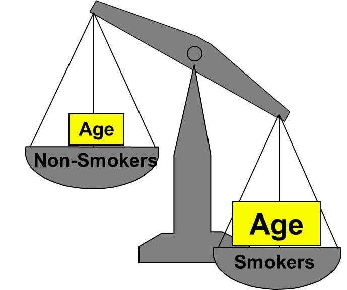

Confounding is a distortion of the association between an exposure and an outcome that occurs when the study groups differ with respect to other factors that influence the outcome. Unlike selection and information bias, which can be introduced by the investigator or by the subjects, confounding is a type of bias that can be adjusted for in the analysis, provided that the investigators have information on the status of study subjects with respect to potential confounding factors.
Effect modification is distinct from confounding; it occurs when the magnitude of the effect of the primary exposure on an outcome (i.e., the association) differs depending on the level of a third variable.
After completing this module, the student will be able to:
Confounding is a distortion (inaccuracy) in the estimated measure of association that occurs when the primary exposure of interest is mixed up with some other factor that is associated with the outcome. In the diagram below, the primary goal is to ascertain the strength of association between physical inactivity and heart disease. Age is a confounding factor because it is associated with the exposure (meaning that older people are more likely to be inactive), and it is also associated with the outcome (because older people are at greater risk of developing heart disease).

In order for confounding to occur, the extraneous factor must be associated with both the primary exposure of interest and the disease outcome of interest. For example, subjects who are physically active may drink more fluids (e.g., water and sports drinks) than inactive people, but drinking more fluid has no effect on the risk of heart disease, so fluid intake is not a confounding factor here.

Or, if the age distribution is similar in the exposure groups being compared, then age will not cause confounding.

Rothman and others use a study by Stark and Mantel to illustrate the key features of confounding. These authors investigated the association between birth order and the risk of Down syndrome. The first graph to the right shows a clear trend toward increasing prevalence of Down syndrome with increasing birth order, or an association between increasing birth order and risk of Down syndrome.
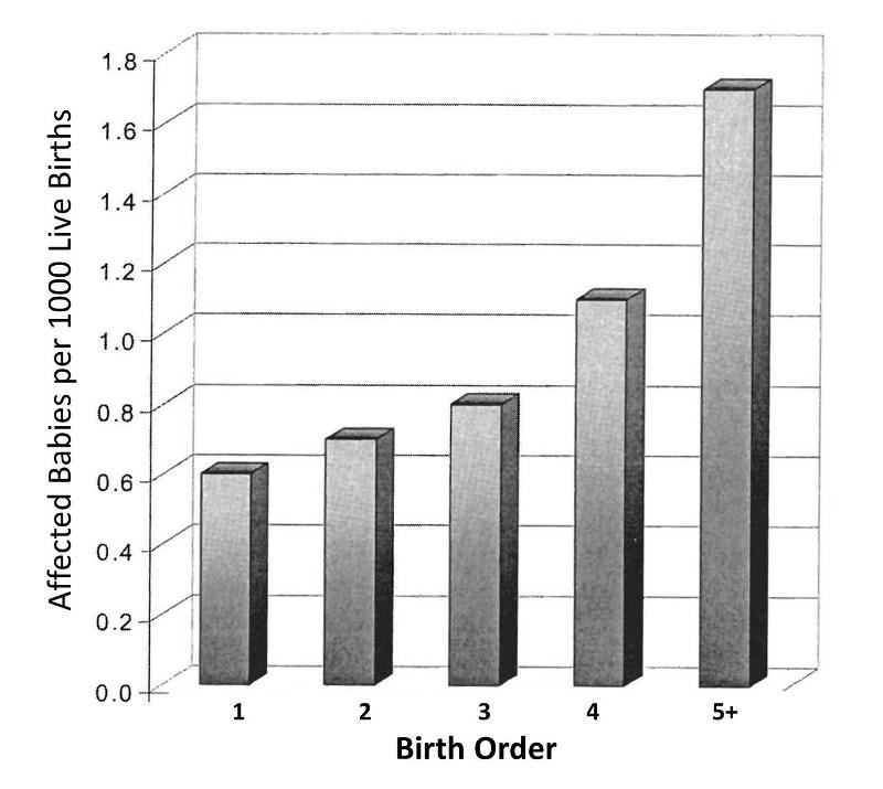
A 5th born child appears to have roughly a 4-fold increase in risk of being born with Down syndrome. Results like this also invite us to think about the mechanisms by which this occurred. Why might birth order cause a greater risk of Down syndrome? Keep in mind that this analysis does not consider any other "risk factors" besides birth order.
However, consider also that the order in which a women's children are born is also linked to her age at the time of her child's birth. When Stark and Mantel examined the relationship between maternal age at birth and risk of the child having Down syndrome, they observed the relationship depicted in the bar graph below. This shows an even more striking relationship between maternal age at birth and the child's risk of being born with Down syndrome.
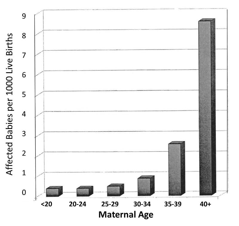
Obviously, women giving birth to their fifth child are on average, older than women giving birth to their first child. In other words, birth order of children is mixed up with maternal age when a child is born. The correlation between maternal age and prevalence of Down syndrome is much stronger than the correlation with birth order, and a woman having her 5th child is clearly older than when she gave birth to her previous children. In view of this, the relationship between birth order and prevalence of Down syndrome is confounded by age. In other words, the association between birth order and Down syndrome is exaggerated by the confounding effect of maternal age.
But is the converse also true? Is the effect of maternal age confounded by birth order? It is possible, but only if birth order really has some independent effect on the likelihood of Down syndrome, i.e. an effect independent of the fact that birth order is linked to maternal age. Rothman points out that a good way to sort this out is to look at both effects simultaneously, as in the graph below.
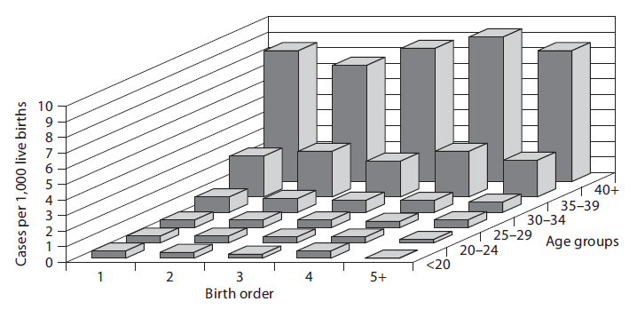
In a sense this graph shows the relationships by stratifying the prevalence of Down syndrome by both birth order and maternal age. If one focuses on how prevalence changes within any particular maternal age group looking from side to side, it is clear that increasing birth order does not correlate with the prevalence of Down syndrome. In other words, if one "controls for maternal age," there is no evidence that birth order has any impact. On the other hand, if one now examines changes in prevalence within each of the birth order groups by looking from front to back within a given birth order, there is clearly a marked increase in prevalence as maternal age increases within all five levels of birth order. In other words, even after taking birth order into account (i.e., controlling for birth order) the strong association with maternal age persists.
Based on this analysis one can conclude that the association between birth order and Down syndrome was confounded by age. The different birth order groups had different age distributions, and maternal age is clearly associated with prevalence of Down syndrome. As a result, the apparent association between birth order and and Down syndrome that was seen in the first figure was completely due to the confounding effect of age. On the other hand, the association between maternal age and Down syndrome was NOT confounded by birth order, because birth order has no impact on the prevalence of Down syndrome, and the association between age and Down was not distorted by differences in birth order.
Most health problems have many determinants ("risk factors"), so it is not surprising that there is a lot of potential for confounding. While this can represent a barrier to testing a particular hypothesis, it is also an opportunity to dissect the many determinants and to define their relative importance.
In "Epidemiology - An Introduction" Ken Rothman says the following about this complexity:
"The research process of learning about and controlling for confounding can be thought of as a walk through a maze toward a central goal. The path through the maze eventually permits the scientist to penetrate into levels that successively get closer to the goal: in [the example of maternal age and Down syndrome] the apparent relations between Down syndrome and birth order can be explained entirely by the effect of mother's age, but that effect in turn will ultimately be explained by other factors that have not yet been identified. As the layers of confounding are left behind, we gradually approach a deeper causal understanding of the underlying biology. Unlike a maze, however, this journey toward biologic understanding does not have a clear endpoint, in the sense that there is always room to understand the biology in a deeper way."
There are three conditions that must be present for confounding to occur:
For example, it is known that modest alcohol consumption is associated with a decreased risk of coronary heart disease, and it is believed that one of the mechanisms by which alcohol causes a reduced risk is that alcohol raises blood levels of HDL, the so called "good cholesterol." Higher levels of HDL are known to be associated with a reduced risk of heart disease. Consequently it is believed that modest alcohol consumption raises HDL levels, and this, in turn, reduces coronary heart disease. In a situation like this HDL levels are not confounder of the association between alcohol and heart disease, because it is part of the mechanism by which alcohol produces this beneficial effect. If increased HDL is a consequence of alcohol consumption and part of the mechanism by which it lowers the risk of heart disease, then it is not a confounder..
![]()
Not surprisingly, since most diseases have multiple contributing causes (risk factors), there are many possible confounders.
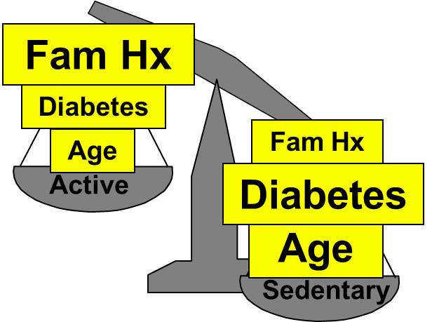
As a result, there may be many possible confounding factors that could influence an association. For example, in looking at the association between exercise and heart disease, other possible confounders might include age, diet, smoking status and a variety of other risk factors that might be unevenly distributed between the groups being compared.
Aside from their physical inactivity, sedentary subjects may be more likely to smoke, to have high blood pressure and diabetes, and to consume diets with a higher fat content; all of these factors would tend to increase the risk of coronary heart disease. On the other hand, subjects who go to a gym regularly (active) may be more likely to be males and perhaps more likely to have a family history of heart disease, i.e., factors that might increase the risk of active subjects. Consequently, there may be many confounders that can distort the estimate of association in one direction or another.
Family History of Heart Disease

The magnitude confounding can be quantified by computing the percentage difference between the crude and adjusted measures of effect. There are two slightly different methods that investigators use to compute this, as illustrated below.
Percent difference is calculated by calculating the difference between the starting value and ending value and then dividing this by the starting value. Many investigators consider the crude measure of association to be the "starting value".
Other investigators consider the adjusted measure of association to be the starting value, because it is less confounded than the crude measure of association.
While the two methods above differ slightly, they generally produce similar results and provide a reasonable way of assessing the magnitude of confounding. Note also that confounding can be negative or positive in value.

Residual confounding is the distortion that remains after controlling for confounding in the design and/or analysis of a study. There are three causes of residual confounding:
Confounding by indication is a special type of confounding that can occur in observational (non-experimental) pharmaco-epidemiologic studies of the effects and side effects of drugs. This type of confounding arises from the fact that individuals who are prescribed a medication or who take a given medication are inherently different from those who do not take the drug, because they are taking the drug for a reason. In medical terminology, such individuals have an "indication" for use of the drug. Even if the study population consists of subjects with the same disease, e.g., osteoarthritis, they may differ in the severity of their disease and may therefore differ in the need for medication. Aschengrau and Seage give the example of studies of the association between antidepressant drug use and infertility. The use of antidepressant medications may appear to be associated with an increased risk of infertility. However, depression itself is a known risk factor for infertility. As a result, there would appear to be an association between antidepressants and infertility. One way of dealing with this is to study the association in subjects who are receiving different treatments for the same underlying disease condition.
A variation on this might be dubbed "confounding by contraindication." For example, in the case-control study by Perneger and Whelton examining the association between analgesic drug use and kidney failure the authors compared prior analgesic use between patients receiving kidney dialysis and population controls without known kidney disease. Suppose that patients on dialysis had been advised to avoid taking aspirin because of its effects on blood clotting; they may have been advised to take acetaminophen (Tylenol) instead). If the group of dialysis cases included a number of people who had been on long-term dialysis, this would result in a decreased frequency of aspirin use and and increased use of Tylenol in the case group. As a result, an association with aspirin would be underestimated, while an association with Tylenol would be overestimated.
Reverse causality occurs when the probability of the outcome is causally related to the exposure being studied. For example, Child feeding recommendations of the World Health Organization include breastfeeding for two years or more, because of evidence that breast fed children have a reduced risk of infectious agents and are less likely to die. However, some studies have produced conflicting concerns. One possibility is that in communities with very poor resources the children who are at greatest risk and perhaps have the least access to other food sources are more likely to be breast fed for at least two years. A comparison of growth and development between these children and more advantaged children would likely find less progress in the breast fed group. (See "Association of Breastfeeding and Stunting in Peruvian Toddlers: An Example of Reverse Causality" by Marquis GS, et al.: International Journal of Epidemiology 1997; 26: 349–356.
The case-control study by Perneger and Whelton may also have been affected by reverse causality. Diabetes is a leading cause of renal failure in the US, and chronic diabetes is associated with a number of other health problems such as cardiovascular diseases and infections that could result in a greater use of analgesics. If so, the dialysis cases whose renal failure resulted from diabetes might have taken more analgesics because of their diabetes. Nevertheless, it would appear that analgesic use was associated with an increased risk of renal failure rather than vice versa.

One of the conditions necessary for confounding to occur is that the confounding factor must be distributed unequally among the groups being compared. Consequently, one of the strategies employed for avoiding confounding is to restrict admission into the study to a group of subjects who have the same levels of the confounding factors. For example, in the hypothetical study looking at the association between physical activity and heart disease, suppose that age and gender were the only two confounders of concern. If so, confounding by these factors could have been avoided by making sure that all subjects were males between the ages of 40-50. This will ensure that the age distributions are similar in the groups being compared, so that confounding will be minimized.
This approach to controlling confounding is simple and effective, but it has several limitations:
Instead of restriction, one could also ensure that the study groups do not differ with respect to possible confounders such as age and gender by matching the two comparison groups. For example, for every active male between the ages of 40-50, we could find and enroll an inactive male between the ages of 40-50. In this way, the groups we are comparing can artificially be made similar with respect to these factors, so they cannot confound the relationship. This method actually requires the investigators to control confounding in both the design and analysis phases of the study, because the analysis of matched study groups differs from that of unmatched studies. Like restriction, this approach is straightforward, and it can be effective. However, it has the following disadvantages:
Nevertheless, matching is useful in the following circumstances:
You previously studied randomization in the online module on Clinical Trials. Given the more detailed discussion in this current module of the conditions necessary for confounding to occur, it should be obvious why randomization is such a powerful method to control prevent confounding. If a large number of subjects are allocated to treatment groups by a random method that gives an equal chance of being in any treatment group, then it is likely that the groups will have similar distributions of age, gender, behaviors, and virtually all other known and as yet unknown possible confounding factors. Moreover, the investigators can get a sense of whether randomization has successfully created comparability among the groups by comparing their baseline characteristics.
One way of identifying confounding is to examine the primary association of interest at different levels of a potential confounding factor. The side by side tables below examine the relationship between obesity and incident CVD in persons less than 50 years of age and in persons 50 years of age and older, separately.
Table of Obesity and Incident Cardiovascular Disease by Age Group